Tag Archives: R

R Groundhog

Reproducible science needs controlled environments.

Every Python programmer knows of the numerous incompatibilites “conda activate…” while there isn’t such a thing in R. Well until now… or at least as I learned it today…

Groundhog should be a R core function.


https://groundhogr.com/

Aug 5, 2023

Thank you for pointing me to renv 1.0.0

We’re thrilled to announce the release of renv 1.0.0. renv has been around since 2019 as the successor to packrat, but this is the first time (!!) we’re blogging about it.

DPI and PPI in scientific publications

It seems that also graphic design tasks are more and more shifted to the authors. A journal asked me to revise my R “figures with >6 px size fonts at 600 dpi” which does not make so much sense to me as it mixes apples and oranges (DPI and PPI) and does even give me any size estimate of the final image.

Fortunately, there is a great website that has a lot of helpful explanations and demo code.

In summary PPI are number of pixels per inch. Pixel is the smallest unit that can be displayed on a screen, the picture x element. So my screen has about 227 ppi which is super sharp while for historical reasons not the physical but a logical PPI of 96 is being assumed for screens. Continue reading DPI and PPI in scientific publications

A R function creating 96 well plate sample assignment

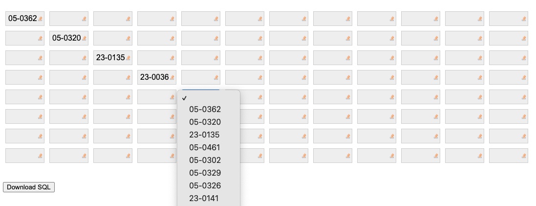
Most recently I had to add forgotten data to a SQL server database that was in use only until 2010. Script language was Cold Fusion at that time creating a visual interface to 96 well plates where proband IDs are assigned to plate positions by drop down fields.

R doesn’t have any good way for formatted data entry. Some shiny apps would be helpful but a bit overkill here. Data export into a javascript framework would be also a more professional solution while I just needed only a quick way to modify my database.

So I came up with some R code producing html code embedding javascript functions that can export the result as SQL code, so a 4 language mixup.

96 well plate assignment
dataentry <- function(plate_id,city) {
# get orig IDs from database first

# position identifier A01, A02...
pos = NULL
for (i in 1:8) {
  pos = c(pos, paste0( rep( LETTERS[i], 12), str_pad( 1:12 ,2,pad="0" ) ) )
}
	
HTML <- paste('<html>
<script>
function download(filename, text) {
  var element = document.createElement("a");
  element.setAttribute("href", "data:text/plain;charset=utf-8," + encodeURIComponent(text));
  element.setAttribute("download", filename);
  element.style.display = "none";
  document.body.appendChild(element);
  element.click();
  document.body.removeChild(element);
}
function saveValues() {
  var frm = document.getElementById("f");
  var params = "";
  var sample_id = ',sample_id,';
  for( var i=0; i<frm.length; i++ ) {
    sample_id++;
    var fieldId = frm.elements[i].id;
    var fieldValue = frm.elements[i].value;
    if (fieldValue) params += "INSERT INTO samples (plate_id,plate_position,patient_id) VALUES (',plate_id,'," + fieldId + "," + fieldValue + ")\\n";
  }
  download("',plate_id,'.SQL",params);
}
</script>
<body>
<form id="f">')
	
# dropdowns
sel ='<option value=""></option>'
for (i in 1:dim(patients)[1]) {
  sel <- paste0(sel,'<option value=',patients[i,"patient_id"],'>',patients[i,"Orig_ID"],'</option>\n')
}
for (i in pos) {
  if (substr(i,2,3) == "01") HTML <- paste0(HTML,'<BR>')
  HTML <- paste(HTML,'<select id=',i,'>',sel,'</select>')
}
	
HTML <- paste(HTML,'</form>
<br><input name="save" type="button" value="SQL" onclick="saveValues(); return false"/>
</body></html>')
	
sink( paste('plate.html') )
cat(HTML)
sink()
}
dataentry(725,'city')

Data and methods available? Forget it!

Bergeat 2022

Data were available for 2 of 65 RCTs (3.1%) published before the ICMJE policy and for 2 of 65 RCTs (3.1%) published after the policy was issued (odds ratio, 1.00; 95% CI, 0.07-14.19; P > .99).

Danchev 2021

Among the 89 articles declaring that IPD would be stored in repositories, only 17 (19.1%) deposited data, mostly because of embargo and regulatory approval.

Gabelica 2022 (visualization @ Nature)

Of 3556 analyzed articles, 3416 contained DAS. The most frequent DAS category (42%) indicated that the datasets are available on reasonable request. Among 1792 manuscripts in which DAS indicated that authors are willing to share their data, 1670 (93%) authors either did not respond or declined to share their data with us. Among 254 (14%) of 1792 authors who responded to our query for data sharing, only 122 (6.8%) provided the requested data.

The same issue applies also to software sharing  where less than 5% of all papers is depositing code. And whenever they deposit software, it is even not running anymore a few years later as operating systems and libraries changed.

Both issues took me many years of my scientific life. It is recognized by politics in Germany but also the most recent action plan looks  … ridiculous. Why not making data and software sharing mandatory at time of publication?

How to scrape a website with R II: WYSIWYG

Part II

Although Rselenium allows a screenshot of the current browser window

library(RSelenium)
remDr <- remoteDriver(
  remoteServerAddr = "localhost",
  port = 4444,
  browserName = "Chrome"
)
remDr$open()
remDr$navigate("http://google.com")
remDr$screenshot(display = T) # remDr$screenshot(file="screen.jpg")

I found it extremely difficult to control a webbrowser running in a Docker container – looking up the DOM tree, injecting javascript etc is a lot of guess work.

So we need also a VNC server in the docker container as found at github.

After starting in the terminal

docker run -d -p 4444:4444 -p 5900:5900 -v /dev/shm:/dev/shm selenium/standalone-chrome:4.0.0-beta-1-prerelease-20210207

we can watch live at vnc://127.0.0.1:5900 what’s going on.

Breaking up long chains in R’s dplyr/magrittr code and calling sub functions

Having several long and redundant chains in R ‘s magittr code, I have now figured out how to pipe into named and unnamed functions

f1 <- function(x) {
  x %>% count() %>% print()
}
f2 <- function(x) {
  x %>% tibble() %>% print()
}

So we have now two named functions with code blocks that can be inserted in an unnamed function whenever needed

iris %>%
  # do any select, mutate ....
  # before running both functions
  (function(x) {
    x %>% select(Species) %>% f1() %>% print()
    x %>% f2() %>% print()
  })

We can make a variable global from inside a function using <<- assignment but I have not found a way to continue the dplyr chain with any returned variable. So we are trapped inside the function

iris %>%
  (function(x) {
    result <<- x %>% head(1)
  })

How to scrape a website with R I: Using a browser generated cookie

While there are quite some SO examples out there how to manage the login, here are the ncessary steps whenever you need to login in manually and have to start with a browser cookie. First install the “EditThisCookie” plugin in Chrome and export the cookie Continue reading How to scrape a website with R I: Using a browser generated cookie

Graphical display of outbreaks: Transmission trees

Let’s start with some examples from the literature, find out necessary elements, compare different versions and develop a R template for general use.

“Exploding Stars”

CDC Field Epidemiology Handbook, 2019, ISBN 9780190933692 p115

“Tetris”

https://doi.org/10.1016/S0140-6736(20)30154-9 (2020)

“Clean Undeterministic”
“Clean Tree”

https://academic.oup.com/mbe/article/34/4/997/2919386

“Tree Addons”

https://openres.ersjournals.com/content/4/2/00162-2017

“Railways”

https://www.ages.at/service/service-presse/pressemeldungen/epidemiologische-abklaerung-am-beispiel-covid-19/

“Simple ”

https://www.ncbi.nlm.nih.gov/pubmed/32003551

“Vertical”

“star bus”

https://en.wikipedia.org/wiki/Index_case

“Mathematical”

https://www.biorxiv.org/content/10.1101/142570v3.full

“Genetics”

https://wwwnc.cdc.gov/eid/article/26/9/20-1798_article

From R to Python

It’s bit confusing if you are having long-term experience with R but need some OpenCV Python code. What worked for me

  1. download and install Python 3.8.3.
  2. pip install opencv-python
  3. pip install opencv-contrib-python
  4. although Spyder or Jupyter is recommended for data science, I went for PyCharm
  5. install Atom and follow the video instructions
  6. take care, numerous non working introductions out there, stick to recent version

R leaflet – keep map in frame after closing info box

Although having some experience with leaflet before, it took me 5 hours to find out how to
(1) change the background color and
(2) re-center my map after the popup was panning the map  basically out view. Here is my solution

leaflet(options = leafletOptions(
 zoomControl = FALSE,
 minZoom=6, maxZoom=6,
 centerFixed = TRUE) ) %>%
addPolygons(data = ds,
 fillColor = ~pal(AnzahlFall),
 color="black", weight = 1,
 fillOpacity = 0.7,
 label = ~name_2,
 popup = ~www,
 popupOptions = popupOptions( autopan=FALSE, keepInView = TRUE ) ) %>%
htmlwidgets::onRender("
 function(el, x) {
  var myMap = this;
  myMap.dragging.disable();
  myMap.on('popupclose', function(e) { myMap.panTo( {lon: 10.26, lat: 51.1} ) });
  var e = document.getElementsByClassName('leaflet-container');
  e[0].style.backgroundColor = 'white';	    
}")

A new animation of the famous HadCRUT4 climate dataset

Download

Here is the R sample code (PPT aspect ratio is 6:4, Youtube wants 16:9) .

As ggplot2 animation packages have major difficulties to manipulate the single frames, I am combining here raw PNGs using ffmpeg.

# read_cru_hemi() modified from https://mccartneytaylor.com/plotting-climate-change-on-a-spider-graph-using-r

list.of.packages <- c("ggplot2", "reshape", "stringr","RColorBrewer")
new.packages <- list.of.packages[!(list.of.packages %in% installed.packages()[,"Package"])]
if(length(new.packages)) install.packages(new.packages)
lapply(list.of.packages, require, character.only = TRUE)

read_cru_hemi <- function(filename) {
  tab <- read.table(filename,fill=TRUE)
  nrows <- nrow(tab)
  hemi <- data.frame(
    year=tab[seq(1,nrows,2),1],
    annual=tab[seq(1,nrows,2),14],
    month=array(tab[seq(1,nrows,2),2:13]),
    cover=array(tab[seq(2,nrows,2),2:13])
  )
  hemi[,15:26][ hemi[,15:26]==0 ] <- c(NA)
  return(hemi)
}

url_dat <- "https://crudata.uea.ac.uk/cru/data/temperature/HadCRUT4-gl.dat"
tempdat <- read_cru_hemi(url_dat)
tempmelt <- melt(tempdat[,c(1,3:14)],id="year")

colfunc <- colorRampPalette(c("grey","grey","red"))
FadeToGrey <- colfunc(2019-1850)

new_theme <- theme_classic() + theme(
  text = element_text(size=18, colour="grey"),
  axis.line = element_blank(), 
  axis.text = element_text(colour="grey"),
  axis.ticks = element_line(colour="grey"),
  axis.title.x = element_blank(),
  panel.border = element_blank(),
  panel.grid.major = element_blank(),
  panel.grid.minor = element_blank(),
  panel.background = element_blank(),
  legend.position = "none"
)
theme_set(new_theme)

for(i in 1850:2019){
p <- ggplot(tempmelt[tempmelt$year %in% 1850:i,], aes(x=variable,y=value,color=as.factor(year),group=year)) + 
  geom_line() +
  scale_x_discrete( labels=month.abb) +
  scale_y_continuous( name="difference from baseline  [ oC ]", limits=c(-1,1) ) +
  annotate("text", x=11, y=1, label=i, size=7) +
  scale_color_manual( values=FadeToGrey[ 1:c(i-1849) ]  )
  fn <- paste("/Users/xxx/Desktop/X/",str_pad(i-1849, 3, pad = "0"),".png",sep="")
  ggsave(p, file=fn, width = 16, height = 9)
}

# not run
# ffmpeg -framerate 10 -i /Users/xxx/Desktop/X/%3d.png -r 5 -pix_fmt yuv420p -y /Users/xxx/Desktop/X/out.mp4


In comparison here is the original circular plot. Would require blue, green, yellow, red in the Color Ramp Palette…


Now it is only a minor step to the warming strips.

ggplot(tempdat, aes(x = year, y = 1, fill = annual))+
  geom_tile()+
  scale_y_continuous(expand = c(0, 0))+
  scale_x_continuous(expand = c(0, 0))+
  scale_fill_gradientn(colors = rev(col_strip)) +
  guides(fill = guide_colorbar(barwidth = 1)) +
  theme( axis.ticks= element_blank(),
         axis.text = element_blank(),
         axis.title = element_blank()
  )

tempmelt$variable <- as.numeric(str_replace(as.character(tempmelt$variable),"month.",""))
ggplot(tempmelt, aes(x = year, y = variable, z = value)) +
  geom_raster(aes(fill = value)) +
  scale_fill_gradientn(colors = rev(col_strip)) +
  scale_x_continuous(expand = c(0,0)) +
  scale_y_continuous(expand = c(0,0)) +
  theme( axis.ticks= element_blank(),
         axis.text = element_blank(),
         axis.title = element_blank()
  )


Rstudio, knitr (Rmarkdown2) and bash

I couldn’t find any example online how to revise my R code getting the exif data from pictures

fn <- c("/usr/local/bin/exiftool /Users/wjst/Desktop/white.tif")
info <- system(fn,inter=TRUE,wait=TRUE)

when moving now to knitr. So here is what worked for me as a replacement including the parsing
of exiftool output.

```{r, engine='bash', echo=FALSE}
/usr/local/bin/exiftool /Users/wjst/Desktop/white.tif >/Users/wjst/Desktop/white.txt
```
```{r Exif, echo=FALSE}
fn <- '/Users/wjst/Desktop/white.txt'
info <- paste(readLines(fn))
info <- strsplit(info,"[:]{1}[ ]{1}")
info <- matrix(data=unlist(info), ncol = 2, byrow = TRUE)
info <- gsub("(^[[:space:]]+|[[:space:]]+$)", "", info)
```
*Exif*
`r kable(info)`

Better figures

A recent paper identifies 10 rules for better pictures. As I have also given several lectures on that topic, I was excited what the authors think…
1. Know your audience. This is trivial as you never know your audience.
2. Identify your message. True and not true at the same time. True as it makes your findings more evident – not true if you are allowing a reader to find his own message.
3. Adapt the figure to the support medium. Trivial. May be very time consuming.
4. Captions are not optional. Absolutely true, I also suppport good captions – mini stories for those who can’t read the whole text.
5. Do not trust the defaults. Trivial. No one does.
6. Use color efficiently.  Not really,  avoid colors for those of us who are colorblind and to avoid expensive page charges.
7. Do not mislead the reader. Why should I?
8.  Avoid Chartjunk. Absolutely. Most frequent problem.
9. Message trumps beauty. Sure, form follows function.
10. Get the right tool. Maybe correct while the further recommendations look like a poor man’s effort to make his first graphic at zero cost: Gimp, Imagemagick, R…