Category Archives: Software

Scientific publishing in the age of interacting AIs

I will not repeat here what I already wrote about author vs journal interaction where I predicted high speed transactions.

What I can share here is an ongoing review process where a reviewer is now using a tool giving me an increasing workload.

Related in silico work has been published by Anthropic scientists recently who asked the agents to peer-review each other’s findings in a “build a game” experiment. They write

When we humans learn new information, we use our discretion in determining how to apply it to future decisions. We might consider the content of the information itself, like how consistent it is with what we already know, or whether it appeals to our values-or we might consider the source, e.g. how historically reliable it has been, and whether it has a vested interest in changing our beliefs. Our world contains deceptive actors, and we need to apply skepticism to guard against them. AI models, however, lack this-and their more brittle epistemics affect their behavior toward humans and toward each other.

AI agents, while broadly knowledgeable, have limited exposure to or defenses against exploitative senders. Most applications test their capabilities in instruction-following settings, where their sole objective is to fulfill users' requests. But accumulated experience is needed to develop intuitions about who is trustworthy. As we move into a regime of multiagent interaction, where the presence of malicious actors is no longer speculative, we wonder: in the right setting, would agents be capable of similar epistemic vigilance?

In the aftermath of the following review I should have included some whitespace LLM instructions as had been done now by a congress organizer [Casrai, Nature]. So the only thing I can share now is a semantic analysis of a reviewer who comments on my farming manuscript.

In rounds 1 and 2 the use of a LLM can be ruled out. There are numerous errors of reviewer #2, of kinds that instruction-tuned models essentially never emit:

  • Homophone substitution: “Where they really excluded?” for “Were”
  • Typos: “invididual”, “persona exposure”, “residental”, “labeled”
  • Number disagreement: “many paper have”, “these comparison”, “criteria … is not specified”
  • Article omission: “Present paper by-passes”, “Author fails”, “may be major reason”, “some of first studies”
  • Infinitive error: “makes the reader to wonder”

Layered on that is a consistent L1-transfer signature pointing to German or Finnish: comma before an embedded interrogative or conditional (“interesting to learn, how fast”, “may be major reason, why classification”, “labeled as stratified, if they were”), the calque “Is it so that …”, German constituent order.

But by the third round the very same reviewer #2 appears unsettled, plausibly because the earlier objections had not landed. The prose changes at exactly that point. Not one of the 56 sentences he wrote in rounds 1 and 2 contains a semicolon; two of his eight round-3 comments do (Fisher exact p = 0.014). Hardly rocket science, but it is a real discontinuity, and the orthography flips alongside it, from repeated “labeled” to “labelled”.

The argument drifts too, with a certain amnesia. In round 2 the complaint was that rural-restricted studies had been wrongly labelled stratified. In round 3 the complaint is that rural-restricted studies have been wrongly labelled representative.

Most striking, a full sentence is carried over from Reviewer 1’s report of the previous round. Reviewer 1 wrote: “strong statements about previous literature, conflicts of interest, and possible publication bias. These points may be relevant, but they should be expressed in a more neutral and evidence-based tone.” In round 3 this reappears, from the anonymous reviewer 2, as: “Strong statements about previous literature, conflicts of interest, and possible publication bias should be expressed in a more neutral and evidence-based tone.”

The evidence is thin, but the round-3 comments read less like a reviewer who has re-read the manuscript than like a reviewer whose remaining objections have been assembled and smoothed by a tool.

So arguing we in future paper submission increasingly against a LLM?

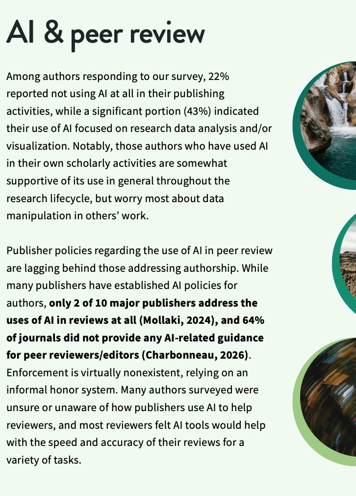
A Frontiers survey of over 1,600 academics found that 53% of peer reviewers have used AI tools in their work. Note also that Springer Nature instructs peer reviewers not to upload manuscripts into generative AI tools, emphasising that manuscripts contain confidential and sensitive information.

BMC Public Health is Springer Nature. If my reviewer #2 pasted my manuscript into a model, that is a policy breach independent of whether the resulting comments were any good.


CC-BY-NC Science Surf , accessed 16.08.2026

Zwei Schichten in der Logienquelle: Eine AI basierte Analyse

Die Logienquelle Q ist ein hypothetisches Dokument: jene rund 235 Verse, welche die Evangelisten MatthÀus und Lukas teilen, ohne dass sie bei Markus stehen. Von den 661 Markus-Versen finden sich etwa 600 bei MatthÀus und rund 350 bei Lukas wieder, wobei die genauen Zahlen je nach ZÀhlweise (wörtliche Parallele oder inhaltliche Entsprechung) schwanken. Diskutiert wird, ob Q noch vor dem Markusevangelium entstanden und zumindest in seinen AnfÀngen in GalilÀa zusammengestellt worden ist.

Als ich 1979 Theologie studierte, war Q nur als singulĂ€rer Corpus bekannt. John Kloppenborg hat dann 1987 eine einflussreiche Schichtenanalyse vorgelegt: Q1 als Ă€ltere weisheitliche Unterweisung (Feldrede, Aussendungsrede, Vaterunser, Sorget-nicht-Worte) und Q2 als spĂ€tere redaktionelle Gerichtsschicht (TĂ€uferpredigt, Beelzebul, Jonazeichen, Weherufe, Menschensohn-Worte), dazu Q3 als spĂ€te ErgĂ€nzung mit der VersuchungserzĂ€hlung. Die These beruht auf literarkritischen Argumenten: charakteristische Formen, charakteristische Motive und impliziertes Publikum. Übereinstimmungsraten zwischen MatthĂ€us und Lukas spielen bei Kloppenborgs Zuordnung keine Rolle, ein Test daran ist also nicht zirkulĂ€r.

Eine unabhĂ€ngige, quantitative ÜberprĂŒfung fehlt meines Wissens; mir war es immer zu aufwendig, Texte einzulesen, n-gram und Übereinstimmungen zu rechnen. FĂŒr Details zum Textbestand siehe das Internationale Q-Projekt im Anhang.

Die ĂŒberprĂŒfbare Hypothese: Wenn Q1 und Q2 unterschiedliche Entstehungs- oder Überlieferungsgeschichten haben, könnte sich das in der wörtlichen Übereinstimmung zwischen MatthĂ€us und Lukas niederschlagen. Diese Übereinstimmung gilt seit langem als bimodal, manche Perikopen sind im Griechischen fast identisch, andere teilen nur den Inhalt. Verteilt sich diese BimodalitĂ€t zufĂ€llig ĂŒber das Material, oder folgt sie den Schichten?

Methode. Textgrundlage ist der SBLGNT (griechischer Text, dekodiert aus einem SWORD-Modul). Klassifiziert wird nach der vers weisen Zuordnung von Kloppenborg: 19 Perikopen Q1, 25 Q2, 1 Q3. FĂŒr jede Perikope wurde die Übereinstimmung zwischen dem Lukas- und dem MatthĂ€ustext berechnet: lĂ€ngste gemeinsame Teilfolge (LCS) auf Wortebene, normalisiert auf die mittlere PerikopenlĂ€nge, sowie der Jaccard-Index gemeinsamer 4-grams. Verglichen wurden die Verteilungen per Mann-Whitney-Test, ergĂ€nzt um einen Permutationstest und Kontrollen fĂŒr LĂ€nge, Gattung und Position im MatthĂ€usevangelium. Der Test ist nicht zirkulĂ€r: Kloppenborgs Einteilung wurde nicht anhand von diesen Übereinstimmungen getroffen.

Als Eichung dient die DreifachĂŒberlieferung. Dort, wo MatthĂ€us und Lukas nachweislich dieselbe erhaltene schriftliche Quelle kopieren, nĂ€mlich Markus, lĂ€sst sich mit derselben Metrik messen, wie das Kopieren einer gemeinsamen Schriftquelle quantitativ aussieht. 27 Perikopen, dieselbe Rechnung.

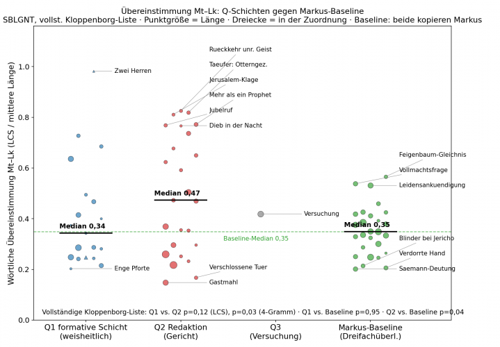
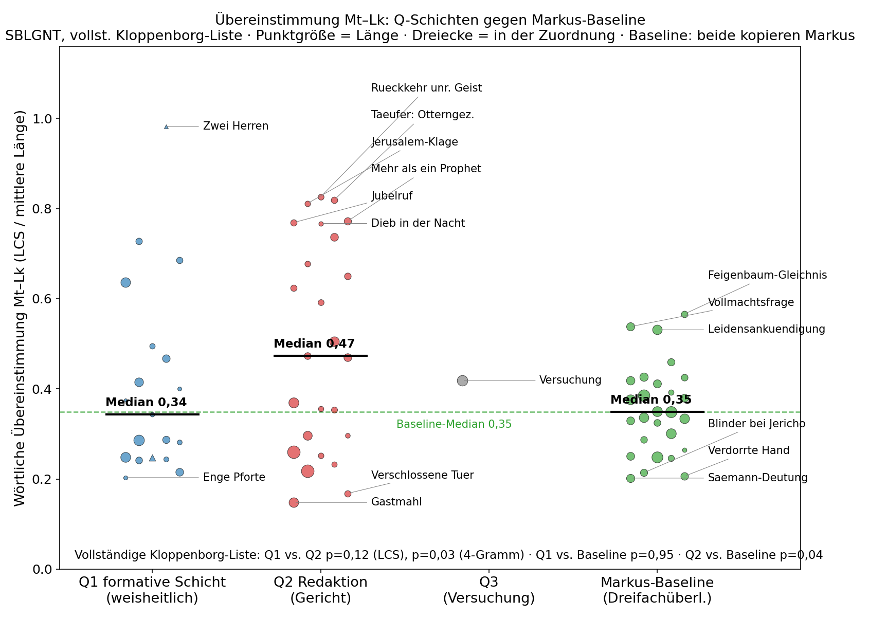
Ergebnis. Die beiden Schichten unterscheiden sich in der Wortlauttreue nicht signifikant. LCS-Übereinstimmung liegt im Median bei 0,34 (Q1) gegen 0,47 (Q2), p = 0,17. Beim 4-gram-Jaccard 0,03 gegen 0,12, p = 0,045, also an der Konventionsgrenze und ohne Korrektur fĂŒr multiples Testen. Was in der DoppelĂŒberlieferung bimodal streut, streut nicht entlang der Schichtgrenze.

Die Markus-baseline liegt bei einem Median von 0,349 (Mt gegen Mk 0,46, Lk gegen Mk 0,43). Die ursprĂŒngliche Erwartung von 0,5 bis 0,6 war falsch, denn die Mt-Lk-Übereinstimmung ist die Schnittmenge zweier unabhĂ€ngiger Redaktionen und liegt damit unter der Treue jeder einzelnen.

Gemessen daran ist Q1 (0,343) von der Baseline statistisch ununterscheidbar. Q1-Material verhĂ€lt sich also exakt so, wie zwei Evangelisten eine gemeinsame schriftliche Quelle mit normaler redaktioneller Freiheit kopieren. Die niedrige Q1-Übereinstimmung ist kein Argument gegen eine Schriftquelle. Q2 (0,473) liegt ĂŒber der Baseline, mit p = 0,043 gerade signifikant.

Interessanter ist eine Grenze quer dazu. Q2 ist intern bimodal. Kurze OrakelsprĂŒche unter 160 Wörtern liegen bei Median 0,62: RĂŒckkehr des unreinen Geistes 0,83, OtterngezĂŒcht-Predigt des TĂ€ufers 0,82, Jerusalem-Klage 0,81, Jubelruf 0,77, Dieb in der Nacht 0,77, treuer Knecht 0,74. Die langen Gleichnisse derselben Schicht liegen bei 0,42 und darunter: Gastmahl 0,15, verschlossene TĂŒr 0,17, Pfunde 0,22. Derselbe Gradient findet sich in Q1 (kurz 0,38, lang 0,29) und in der Markus-Baseline, wo die spruchlastigsten Perikopen die Liste anfĂŒhren (Feigenbaum-Gleichnis 0,57, Vollmachtsfrage 0,54, LeidensankĂŒndigung 0,53) und reine ErzĂ€hlung bei 0,2 bis 0,4 liegt.

Interpretation. Die Überlieferungstreue folgt mehr Form und LĂ€nge, nicht der Schicht. Kurze, stark strukturierte prophetische Rede mit Parallelismen und Reihungen lĂ€sst sich nicht paraphrasieren, ohne sie zu zerstören – sie wird also zitiert, nicht nacherzĂ€hlt. Lange ErzĂ€hlgleichnisse und Mahnrede werden umformuliert. Beide Evangelisten haben denselben Reflex, und deshalb bleibt die Schnittmenge bei formelhaftem Kurzmaterial hoch, unabhĂ€ngig davon, aus welcher Schicht es stammt. Dass die Weherufe gegen die PharisĂ€er, ein KernstĂŒck von Q2, mit 0,26 zu den niedrigsten Werten ĂŒberhaupt gehören, passt: es ist der lĂ€ngste Block im ganzen Material.

Damit stĂŒtzt die Messung die Zwei-Schichten-Hypothese nicht unbedingt. Sie widerlegt sie auch nicht, denn Kloppenborgs Argumente sind literarkritisch und stehen oder fallen nicht an Wortlautstatistik. Sie hĂ€tte eine Signatur haben können, aber ich finde keine. Unter der Farrer-Hypothese (Lukas benutzt MatthĂ€us, kein Q) lesen sich dieselben Zahlen ohnehin genauso: Lukas zitiert kurze Gerichtsworte wörtlich und baut lange ErzĂ€hlstĂŒcke um. Die Messung diskriminiert nicht zwischen gemeinsamer Quelle und direkter AbhĂ€ngigkeit, sie ist kein Existenzbeweis fĂŒr Q, keine Datierung und keine Richtungsentscheidung.

Bemerkenswert bleibt aber der Q1-Befund. Q1 ist fast reines Spruchmaterial, liegt aber auf dem Niveau, das MatthĂ€us und Lukas dem Markus-ErzĂ€hlstoff angedeihen ließen, also niedrig fĂŒr Spruchgut. Ob das an einer variantenreicheren Vorgeschichte liegt, an divergenten Rezensionen, an unabhĂ€ngigen Übersetzungen aramĂ€ischer Vorlagen oder schlicht daran, dass ParĂ€nese Gebrauchstext ist, lĂ€sst sich mit dieser Methode nicht entscheiden.

EinschrĂ€nkungen. Die Baseline setzt voraus, dass beiden Evangelisten ein Markustext nahe dem kanonischen vorlag. Die Diskussion um Proto- und Deuteromarkus und die minor agreements stellt das in Frage. Die Metrik setzt schließlich eine gemeinsame griechische Vorlage voraus.

Anzumerken ist, dass Markus Tiwald in seiner EinfĂŒhrung von 2016 die Kloppenborg-Stratigraphie nicht ĂŒbernimmt. Er spricht von Wachstumsringen in Q, von schriftlichen Vorstufen und von “secondary orality” und löst die Unterscheidung weisheitlich gegen prophetisch als zwei Aspekte derselben Sichtweise auf, nicht als zwei Schichten. Die PrĂ€misse dieses Tests ist also im deutschsprachigen Schrifttum keineswegs Konsens.

Alle Analyse Skripte (SWORD-Dekoder, Analysepipeline, Markus-Baseline) stehen hier zur VerfĂŒgung im Repository. Und hier die verwendete Literatur

  1. Arnal, William E., “The Rhetoric of Marginality: Apocalypticism, Gnosticism, and Sayings Gospels”, Harvard Theological Review 88 (1995) 471-494. EnthĂ€lt in Anm. 12 die hier verwendete versweise Tabellierung der Kloppenborg-Schichten. Cambridge Core
  2. Carlston, Charles E. / Norlin, Dennis A., “Once More: Statistics and Q”, Harvard Theological Review 64 (1971) 59-78.
  3. Carlston, Charles E. / Norlin, Dennis A., “Statistics and Q: Some Further Observations”, Novum Testamentum 41 (1999) 108-123.
  4. Goodacre, Mark, The Case Against Q: Studies in Markan Priority and the Synoptic Problem, Harrisburg 2002.
  5. Holmes, Michael W. (Hg.), The Greek New Testament: SBL Edition, Society of Biblical Literature / Logos Bible Software 2010. Einleitung unter sblgnt.com/about/introduction
  6. Howes, Llewellyn, “Make an Effort to Get Loose: Reconsidering the Redaction of Q 12:58-59”, Pharos Journal of Theology 98 (2017). Volltext (PDF)
  7. Ingolfsland, Dennis, “Kloppenborg’s Stratification of Q and Its Significance for Historical Jesus Studies”, Journal of the Evangelical Theological Society 46/2 (2003) 217-232. Volltext (PDF)
  8. Kloppenborg, John S., The Formation of Q: Trajectories in Ancient Wisdom Collections, Philadelphia 1987. Google Books
  9. Kloppenborg Verbin, John S., Excavating Q: The History and Setting of the Sayings Gospel, Minneapolis 2000.
  10. Robinson, James M. / Hoffmann, Paul / Kloppenborg, John S. (Hg.), The Critical Edition of Q, Leuven / Minneapolis 2000.
  11. Tiwald, Markus, Die Logienquelle. Text, Kontext, Theologie, Stuttgart 2016. doi:10.17433/978-3-17-025628-6
  12. Q-Bibliographie mit Volltextnachweisen: reconstructingq.com


CC-BY-NC Science Surf , accessed 16.08.2026

In the AI era, we will always have to fight for the truth

In the AI era, we will always have to fight for the truth / Das Zeitalter der KI wird ein stÀndiger Kampf um die Wahrheit prÀgen (Jonas Schaible, 2026).

The problem is concrete: AI can be poisoned easily, as we found and now others have replicated. Evidence abounds in the collection of the weirdest images ever published in academic journals.

Meanwhile, the AI optimism narrative persists. A new Science editorial by Holden Thorp documents the gap between promise and practice: “AI in scientific publishing: Slower, worse, and more expensive.” The promises remain seductive –

how it will transform work, claiming that so little human effort will be required that humanity will enter an era of radical abundance, free from disease, drudgery, and danger, among other benefits

yet empirical reality suggests otherwise. Bergstrom et al show that “The unintended consequences of large language models as a labor-augmenting technology in science” actually cut against the optimistic case:

By allowing scientists to work more quickly, LLMs raise the opportunity cost of researcher time, creating incentives to refine papers less thoroughly before moving on. Enticing as it is to imagine that, by saving us time on mundane tasks, LLMs will provide us with more time to think deeply and develop projects completely, our results temper such hopes.

The implication is stark: fighting for truth may now require more labor, not less.


CC-BY-NC Science Surf , accessed 16.08.2026

Time to re-visit Naomi Klein

This is certainly one of the strongest AI pieces ever written: AI machines aren't 'hallucinating'. But their makers are,

She writes

The trick, of course, is that Silicon Valley routinely calls theft "disruption" - and too often gets away with it. We know this move: charge ahead into lawless territory; claim the old rules don't apply to your new tech; scream that regulation will only help China - all while you get your facts solidly on the ground… We saw it with Google's book and art scanning. With Musk's space colonization. With Uber's assault on the taxi industry. With Airbnb's attack on the rental market. With Facebook's promiscuity with our data.

Must read also Lila Shroff

Plenty of people are seemingly starting to feel like depleted AI babysitters… workers were experiencing "mental fatigue from excessive use or oversight of
AI tools beyond one's cognitive capacity.


CC-BY-NC Science Surf , accessed 16.08.2026

My last visit to Stack Overflow

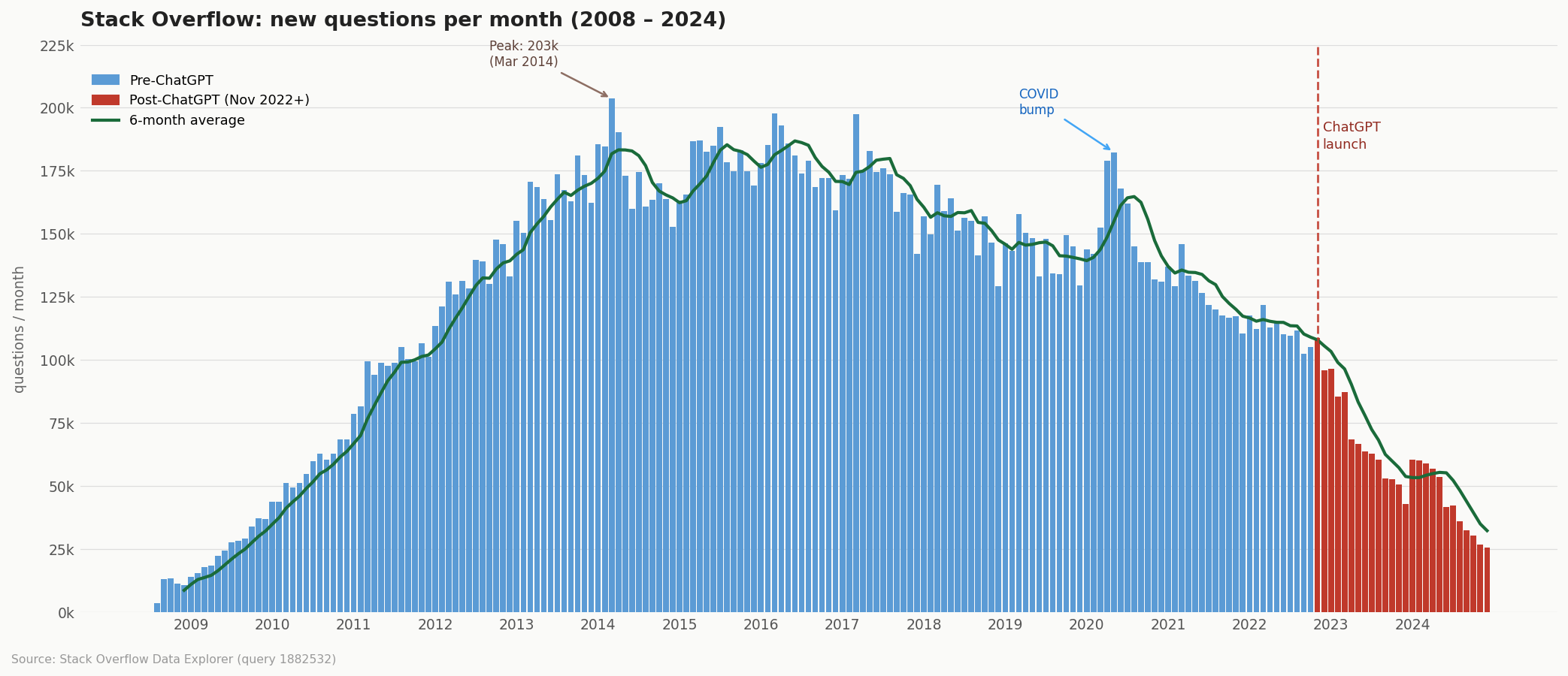
Coding with AI has a nice chart, that I am redrawing here


data source https://data.stackexchange.com/stackoverflow/query/1882532/questions-per-month


so it is time to say Good-Bye now after 14 years

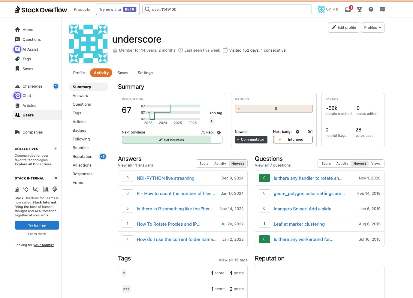
Screenshot 23/3/26 Last Visit to SO

and sticking to the new 10 commandments by Russell Poldrack

Gather Domain Knowledge Before Implementation
Distinguish Problem Framing from Coding
Choose Appropriate AI Interaction Models
Start by Thinking Through a Potential Solution
Manage Context Strategically
Implement Test-Driven Development with AI
Leverage AI for Test Planning and Refinement
Monitor Progress and Know When to Restart
Critically Review Generated Code
Refine Code Incrementally with Focused Objectives


CC-BY-NC Science Surf , accessed 16.08.2026

Is there a data agnostic method to find repetitive data in clinical trials?

There is an interesting observation by Nick Brown over at Pubpeer who analysed a clinical dataset (see also my comment atthe BMJ)

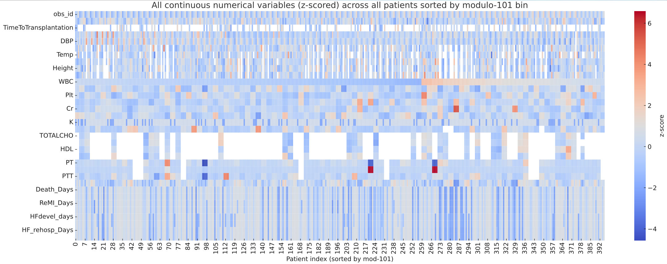
…there is a curious repeating pattern of records in the dataset. Specifically, every 101 records, in almost every case the following variables are identical: WBC, Hb, Plt, BUN, Cr, Na, BS, TOTALCHO, LDL, HDL, TG, PT, INR, PTT

which is remarkable detective work. By plotting the full dataset as a heatmap of z scores, I can confirm his observation of clusters after sorting for modulo 101 bin.

How could we have found the repetitive values without knowing the period length? Is there any formal, data-agnostic detection method?

If we even don’t know the initial sorting variable, it may makes sense to look primarily for monotonic and nearly unique variables, i.e. that are plausible ordering variables. Clearly, that’s obs_id in the BMJ dataset.

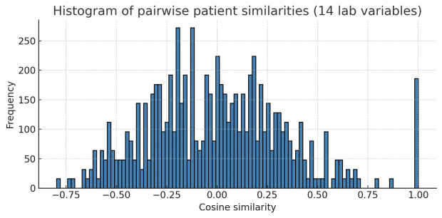
Let us first collapse all continuous variables of a row into a string forming a fingerprint. Then we compute pairwise correlations (or Euclidean distances in this case) of all fingerprints. If a dataset contains many identical or near-identical rows, we will see a multimodal distribution of correlations plus an additional big spike at 1.0 for duplicated rows. This is exactly what happens here.

Unfortunately this works only when mainly repetitive variables are included and not too many non repetitive variables.

Next, I thought of Principal Component Analysis (PCA) as the identical blocks may create linear dependencies and the covariance matrix is becoming rank-deficient. But unfortunately results here were not very impressive – so we better stick with the cosine similarity above.

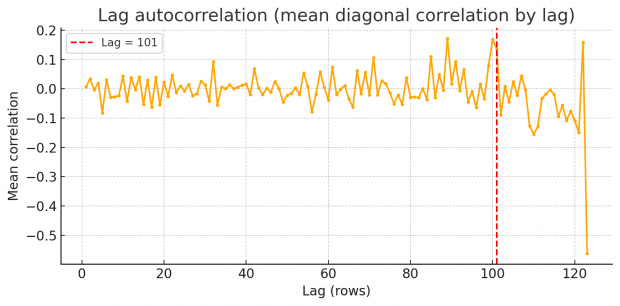
So rest assured we find an excess of identical values, but how to proceed? Duplicates spaced by a fixed lag will cause an high lag k autocorrelation in each variable. Scanning k=1...N/2 reveals spikes at the duplication lag as shown by a periodogram of row-wise similarity in the BMJ dataset.

So there are peaks at around 87, 101 and 122. Unfortunately I am not an expert in time series or signal processing analysis. Can somebody else jump in here and provide some help with FFT?

There may be even an easier method, using the fingerprint-gap . For every fingerprint that occurs more than once, we sort those rows by obs_id and compute the differences of obs_id between consecutive matches. Well, this shows just one dominant gap at 101 only!

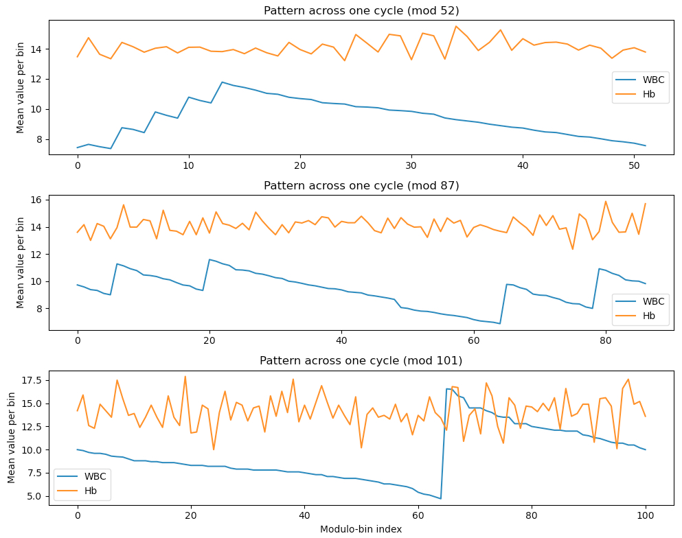
We could test also all relevant mod values, lets say between 50 and 150. For each candidate we compute the across-group variance of the standardized lab-means. The result is interesting

Modulus 52: variance = 0.084019
Modulus 87: variance = 0.138662
Modulus 101: variance = 0.789720

As a cross check let us look into white blood cell counts (WBC) and hemoglobin (Hb).

I am not sure, how to interpret this. Mod 52 may reflect shorter template fragments but did not show up in the autocorrelation test. Mod 87 has rather smooth, coherent curve and is supported by autocorrelation. Mod 101 is more noisy, but gives probably the best explanation for block copying values. Maybe the authors block copied at two occasions?

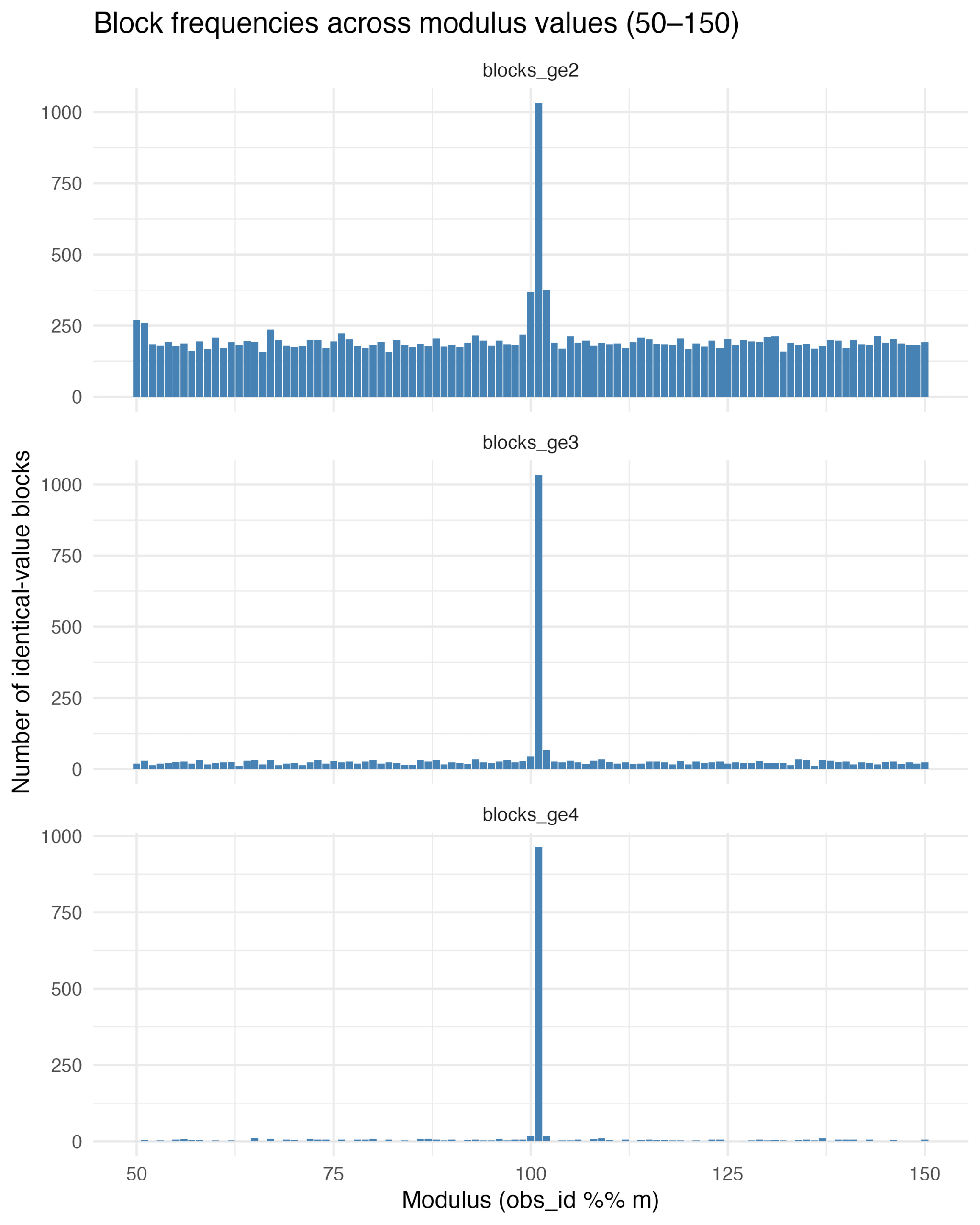
On the next day, I thought of a strategy to find the exact repetition numbers. Why not looping over mod 50 through 150 and just count the number of identical blocks? This is very informative – blocks of size 2, size 3 and 4 or greater show an exact maximum at modulus 101.


23.3.2026 Appendix

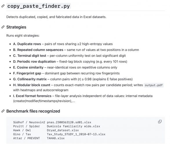
There seems many more studies out there with copy-pastein signs including a Parkinson Cell paper, a PLoS Genetics toxicology paper and a Nat Comm fish ecology study. Here is the Github link to the implementation by Markus Eglund

Hopefully I get the pipeline right by summarizing the entropy calculation there. This is not Shannon entropy – it is a custom measure of how informationally surprising a raw number is. The logic is:

  • Strip the decimal point and trailing zeros from the number’s string representation, then take the absolute integer value. So 0.314 → 314, 0.500 → 5 (trailing zeros stripped), 2016 → 16 (year exception: years 1900-2030 get a capped entropy of 100).
  • Apply a log-scaled transformation: values below 100 get log10(value); values up to 100,000 get 5×log10 - 8; larger values get log10 + 12.
  • For column sequences, sum the individual entropy scores of each value in the run.
  • Adjust downward for “regularity” – if the values in a sequence follow a regular arithmetic interval (e.g. 1.0, 2.0, 3.0), the score is reduced proportionally, because regular sequences can appear legitimately.
  • Normalise by logNumberCountModifier (log of the total number of numeric cells on the sheet) so large sheets don’t get disproportionately penalised.

The suspicion grades are fixed thresholds on the resulting normalized score. I will add the strategy to my Python script (it is implemented here in type script) as another module and upload to Github once it has been sufficiently tested.

31.3.2026 Appendix

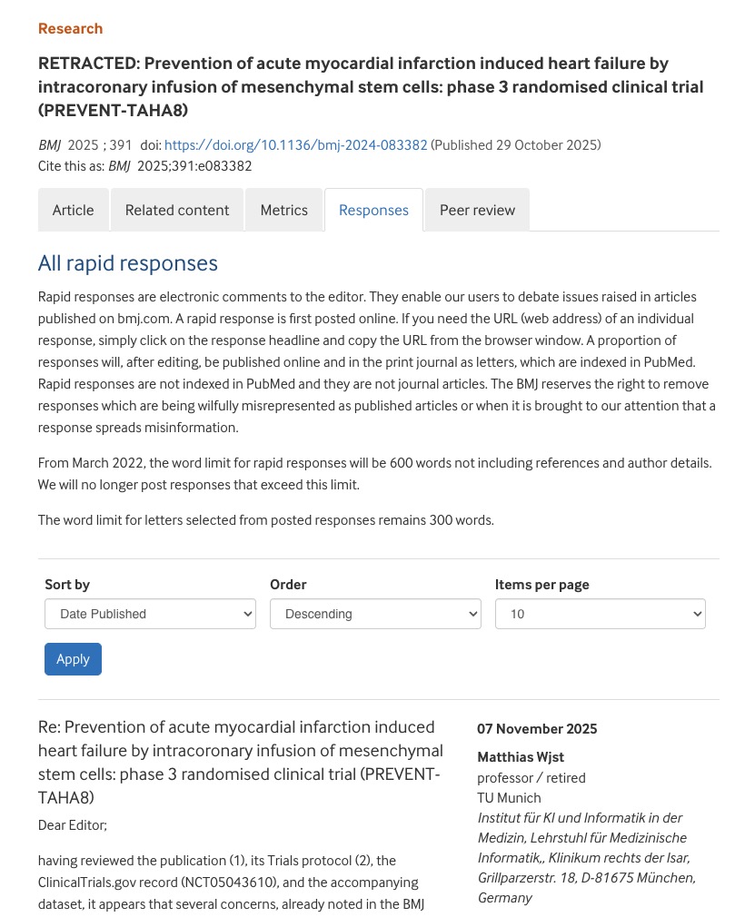
PREVENT-TAHA8, the starting point of this analysis, has been retracted today. I will give a presentation on the avalanche, that has been triggered by this paper, on 29-31 July 2026 in Hannover.

Screenshot 31/3/26


CC-BY-NC Science Surf , accessed 16.08.2026

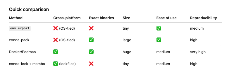
Portable conda – a pain

# v1
conda env export --from-history > environment.yml
conda env create -f environment.yml

# v2
conda install conda-pack
conda pack -n myenv -o myenv.tar.gz
# on target system
mkdir -p ~/envs/myenv && tar -xzf myenv.tar.gz -C ~/envs/myenv
./bin/conda-unpack

# v3
www.docker.com

# v4
micromamba env export / micromamba pack


CC-BY-NC Science Surf , accessed 16.08.2026

A forensic analysis of the Prince Andrew/Giuffre/Maxwell image

There are only a few photographs that made headlines recently. One is Man Ray’s Le Violon d’Ingres for its price tag of $12,400,000.

Or the authorship discussion around the “Napalm Girl” Phan Thị Kim PhĂșc.

And there is a third photograph – a snapshot from a London townhouse two decades ago – that has a similar price tag attached like Le Violon d’Ingres.


My recent paper at https://arxiv.org/abs/2507.1223 examines this infamous photograph using the latest image analysis techniques.

This study offers a forensic assessment of a widely circulated photograph featuring Prince Andrew, Virginia Giuffre, and Ghislaine Maxwell – an image that has played a pivotal role in public discourse and legal narratives. Through analysis of multiple published versions, several inconsistencies are identified, including irregularities in lighting, posture, and physical interaction, which are more consistent with digital compositing than with an unaltered snapshot. While the absence of the original negative and a verifiable audit trail precludes definitive conclusions, the technical and contextual anomalies suggest that the image may have been deliberately constructed. Nevertheless, without additional evidence, the photograph remains an unresolved but symbolically charged fragment within a complex story of abuse, memory, and contested truth.

I provide also a 3D reconstruction of the scene in the preprint although some people may find it easier to watch a video instead.

Even after completion of the analysis there are many open questions – where is the original headshot? There are numerous similar images at various image archives while I have not found any 100% original copy so far.

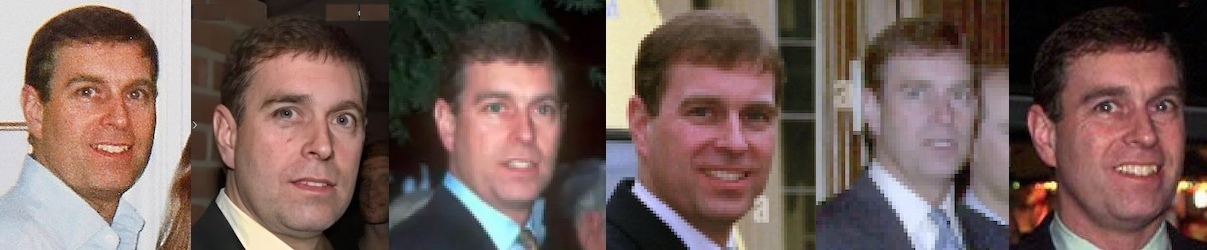
Andrew Mountbatten candidates
Ghislaine Maxwell candidates

Even as there are now reasonable doubts on the image, Prince Andrew could have of course met Virginia Giuffre. Maybe like an artist is painting a scene from memory, this photograph could be showing a real scene although clearly not in a physical sense.

So, to repeat my last sentence in the paper – this photograph remains an unresolved but symbolically charged fragment within a complex story of abuse, memory, and contested truth.

Bonus Link


Note added March 2, 2026

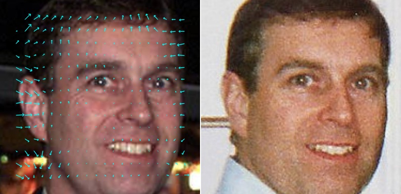
Will add an update to the preprint in the next week as there are some interesting new results from the a comparative analysis of the above images.

the left image seems is the candidate source depicted are the necessary warping transformations.
Flash. highlights


CC-BY-NC Science Surf , accessed 16.08.2026

Attention is all you need

Here is the link to the famous landmark paper in the recent history https://arxiv.org/abs/1706.03762


Before this paper, most sequence modeling (e.g., for language) used recurrent neural networks (RNNs) or convolutional neural networks (CNNs). These had significant limitations, such as a difficulty with long-range dependencies and slow training due to sequential processing. The Transformer replaced recurrence with self-attention, enabling parallelization and faster training, while better capturing dependencies in data. So the transformer architecture became the foundation for nearly all state-of-the-art NLP models. This enabled training models with billions of parameters, which is key to achieving high performance in AI tasks.


CC-BY-NC Science Surf , accessed 16.08.2026

LLM word checker

The recent Science Advance paper by Kobak et al. studied

vocabulary changes in more than 15 million biomedical abstracts from 2010 to 2024 indexed by PubMed and show how the appearance of LLMs led to an abrupt increase in the frequency of certain style words. This excess word analysis suggests that at least 13.5% of 2024 abstracts were processed with LLMs.

Although they say that the analysis was performed on the corpus level and cannot identify individual texts that may have been processed by a LLM, we can of course check the proportion of LLM words in a text.

Unfortunately their online list contains stop words that I am eliminating here. But then we can run the following script!

# based on https://github.com/berenslab/llm-excess-vocab/tree/main

import csv
import re
import os
from collections import Counter
from striprtf.striprtf import rtf_to_text
from nltk.corpus import stopwords
import nltk
import chardet

# Ensure stopwords are available
nltk.download('stopwords')

# Paths
rtfd_folder_path = '/Users/x/Desktop/mss_image.rtfd' # RTFD is a directory
rtf_file_path = os.path.join(rtfd_folder_path, 'TXT.rtf') # or 'index.rtf'
csv_file_path = '/Users/x/Desktop/excess_words.csv'

# Read and decode the RTF file
with open(rtf_file_path, 'rb') as f:
raw_data = f.read()

# Try decoding automatically
encoding = chardet.detect(raw_data)['encoding']
rtf_content = raw_data.decode(encoding)
plain_text = rtf_to_text(rtf_content)

# Normalize and tokenize text
words_in_text = re.findall(r'\b\w+\b', plain_text.lower())

# Remove stopwords
stop_words = set(stopwords.words('english'))
filtered_words = [word for word in words_in_text if word not in stop_words]

# Load excess words from CSV
with open(csv_file_path, 'r', encoding='utf-8') as csv_file:
reader = csv.reader(csv_file)
excess_words = {row[0].strip().lower() for row in reader if row}

# Count excess words in filtered text
excess_word_counts = Counter(word for word in filtered_words if word in excess_words)

# Calculate proportion
total_words = len(filtered_words)
total_excess = sum(excess_word_counts.values())
proportion = total_excess / total_words if total_words > 0 else 0

# Output
print("\nExcess Words Found (Sorted by Frequency):")
for word, count in excess_word_counts.most_common():
print(f"{word}: {count}")

print(f"\nTotal words (without stopwords): {total_words}")
print(f"Total excess words: {total_excess}")
print(f"Proportion of excess words: {proportion:.4f}")

7 Aug 2025

The long ’em dash’ - U+2014 instead of the standard minus – seems to be a characteristic sign of chatGPT 4 even when asked not use it.


CC-BY-NC Science Surf , accessed 16.08.2026

How to sync only Desktop to iCloud

After giving up Nextcloud – which is now overkill for me with 30.000 files of basic setup – I am syncing now using iCloud. As I am working only on the desktop, it would make sense to sync the desktop in regular intervals but unfortunately this can be done only together with the Documents folder (something I don’t want). SE has also no good solution, so here is mine

# make another Desktop in iCloud folder
mkdir -p ~/Library/Mobile\ Documents/com~apple~CloudDocs/iCloudDesktop

# sync local Desktop
rsync -av --delete ~/Desktop/ ~/Library/Mobile\ Documents/com~apple~CloudDocs/iCloudDesktop/

# and run it every hour or so
# launchctl load ~/Library/LaunchAgents/launched.com.desktop.rsync.plist

<?xml version="1.0" encoding="UTF-8"?>
<!DOCTYPE plist PUBLIC "-//Apple//DTD PLIST 1.0//EN" "http://www.apple.com/DTDs/PropertyList-1.0.dtd">
<plist version="1.0">
  <dict>
    <key>KeepAlive</key>
    <dict>
      <key>Crashed</key>
      <true/>
    </dict>

    <key>Label</key>
    <string>launched.com.desktop.rsync</string>

    <key>ProgramArguments</key>
    <array>
      <string>/usr/bin/rsync</string>
      <string>-av</string>
      <string>--delete</string>
      <string>/Users/xxx/Desktop/</string>
      <string>/Users/xxx/Library/Mobile Documents/com~apple~CloudDocs/iCloudDesktop/</string>
    </array>

    <key>RunAtLoad</key>
    <true/>

    <key>StartCalendarInterval</key>
    <array>
      <dict>
        <key>Minute</key>
        <integer>0</integer>
      </dict>
    </array>

    <key>StandardOutPath</key>
    <string>/tmp/rsync.out</string>

    <key>StandardErrorPath</key>
    <string>/tmp/rsync.err</string>
  </dict>
</plist>


CC-BY-NC Science Surf , accessed 16.08.2026

Are we really thinking at 10 bits/s?

There is a funny paper at arXiv, that is now published in Neurology. It claims to have found a

neural conundrum behind the slowness of human behavior. The information throughput of a human being is about 10 bits/s. In comparison, our sensory systems gather data at ~10^9 bits/s. The stark contrast between these numbers remains unexplained and touches on fundamental aspects of brain function: What neural substrate sets this speed limit on the pace of our existence? Why does the brain need billions of neurons to process 10 bits/s? Why can we only think about one thing at a time?

If there are really two brains, an “outer” brain with fast high-dimensional sensory and motor signals and an “inner” brain that does are the processing? My inner brain says this is a huge speculation.


CC-BY-NC Science Surf , accessed 16.08.2026

How to run LLaMA on your local PDFs

I needed this urgently for indexing PDFs as Spotlight on the Mac is highly erratic after all this years.

Anything LLM seemed the most promising approach with an easy to use GUI and being well documented. But indexing failed after several hours, so I went on with LM Studio. Also this installation turned out to be more complicated than expected due to library “dependency hell” and version mismatch spiralling…

  1. Download and install LM Studio
  2. From inside LM Studio download your preferred model
  3. Index your PDFs in batches of 1,000 using the Python script below
  4. Combine indices and run queries against the full index

30.000 PDFs result in a 4G index while the system is unfortunately not very responsive (yet)

Continue reading How to run LLaMA on your local PDFs


CC-BY-NC Science Surf , accessed 16.08.2026

Fighting AI with AI

Here is our newest paper – a nice collaboration with Andrea Taloni et al. along with a nice commentary – to recognize surgisphere-like fraud

Recently, it was proved that the large language model Generative Pre-trained Transformer 4 (GPT-4; OpenAI) can fabricate synthetic medical datasets designed to support false scientific evidence. To uncover statistical patterns that may suggest fabrication in datasets produced by large language models and to improve these synthetic datasets by attempting to remove detectable marks of nonauthenticity, investigating the limits of generative artificial intelligence.

[…] synthetic datasets were produced for 3 fictional clinical studies designed to compare the outcomes of 2 alternative treatments for specific ocular diseases. Synthetic datasets were produced using the default GPT-4o model and a custom GPT. Data fabrication was conducted in November 2024. Prompts were submitted to GPT-4o to produce 12 "unrefined" datasets, which underwent forensic examination. Based on the outcomes of this analysis, the custom GPT Synthetic Data Creator was built with detailed instructions to generate 12 "refined" datasets designed to evade authenticity checks. Then, forensic analysis was repeated on these enhanced datasets. […]

Sufficiently sophisticated custom GPTs can perform complex statistical tasks and may be abused to fabricate synthetic datasets that can pass forensic analysis as authentic.


CC-BY-NC Science Surf , accessed 16.08.2026